nos.tlplotR is an open-source R package for visualizing Newcastle-Ottawa Scale (NOS) risk-of-bias assessments in systematic reviews and meta-analyses — the official R interface to nos-tlplot. It produces publication-ready traffic-light plots and thirteen specialized visualizations:
| Function | Plot |
|---|---|
plot_all() |
Every plot at once |
plot_nos_visualization() |
NOS visualization grid (item-level traffic-light grid with domain bands and totals) |
plot_traffic_light() |
Classic traffic-light bubble plot |
plot_domain_radar() |
Domain radar chart (up to 5 studies) |
plot_theme_radar() |
Theme radar chart (up to 5 studies) |
plot_domain_heatmap() |
Domain-level risk heatmap |
plot_item_heatmap() |
Item-level star heatmap with domain bands |
plot_dot_profile() |
Stacked domain stars per study |
plot_score_table() |
Summary table of stars and overall risk |
plot_donut() |
Risk donut chart per domain |
plot_star_matrix() |
Item-level star ratings matrix |
plot_lollipop() |
Total score lollipop chart |
plot_risk_pie() |
Overall risk-of-bias pie chart |
plot_stacked_area() |
Stacked area risk chart |
Contents
- Installation
- Python setup
- Quick start
- See it in action
- How to use nos.tlplotR in R
- Input data reference
- Themes and output formats
- Return values
- Seeing the Python messages
- Using plots in R Markdown and Quarto
- Bundled example data
- Troubleshooting
- Example gallery
- Citation
- Related links
Installation
Development version from GitHub
# install.packages("pak")
pak::pak("nos-tlplot/nos.tlplotR")

# or
# install.packages("remotes")
remotes::install_github("nos-tlplot/nos.tlplotR")
From a source tarball
install.packages("nos.tlplotR_0.3.0.tar.gz", repos = NULL, type = "source")Install the Python backend manually
nos.tlplotR calls the Python package nos-tlplot. If you prefer to manage Python yourself, install it into the interpreter that reticulate uses:
reticulate::py_install("nos-tlplot", pip = TRUE)or from a terminal:
Python setup
nos.tlplotR requires Python >= 3.12 and nos-tlplot >= 3.0.2. The version is a minimum: pip installs the newest release that satisfies it. You have three options.
Option 1: Let reticulate manage Python (easiest)
On load, nos.tlplotR declares its Python dependency with reticulate::py_require("nos-tlplot>=3.0.2"). If no other Python installation is found, reticulate creates a managed environment and installs nos-tlplot (plus numpy, pandas, matplotlib, seaborn, pyarrow, openpyxl and Pillow) the first time you create a plot. The first call therefore takes a few minutes; later calls are fast because the environment is cached.
library(nos.tlplotR)
plot_nos_visualization(system.file("extdata", "sample_nos.csv", package = "nos.tlplotR"), "nos.png")
Option 2: Use an existing virtual environment or conda environment
reticulate::virtualenv_create("nos-tlplot-env", packages = "nos-tlplot")
reticulate::use_virtualenv("nos-tlplot-env", required = TRUE)

# or
reticulate::conda_create("nos-tlplot-env", packages = "nos-tlplot")
reticulate::use_condaenv("nos-tlplot-env", required = TRUE)
Call use_virtualenv() / use_condaenv() before the first plot call in the session.
Option 3: Use a specific system Python
Sys.setenv(RETICULATE_PYTHON = "/path/to/python3")To make this permanent, add the same line to your ~/.Renviron, then restart R. Alternatively use reticulate::use_python("/path/to/python3", required = TRUE).
Verify the setup
reticulate::py_config()                      # which interpreter is used
reticulate::py_module_available("nos_tlplot") # must be TRUE
py_config() also prints the versions of Python and reticulate that you should include when reporting a problem.
If Python itself is missing, reticulate can install one:
reticulate::install_python()Quick start
library(nos.tlplotR)

# Create the NOS visualization plot from the bundled example file
out <- plot_nos_visualization(
  input_file  = system.file("extdata", "sample_nos.csv", package = "nos.tlplotR"),
  output_file = "nos.png"
)

out
#> [1] "/path/to/nos.png"
Open nos.png with any image viewer, or inside R:
utils::browseURL(out)See it in action
Each plot below was created by a live R session from the bundled example data. The console shows the exact calls; the figure underneath is the file the function returned.
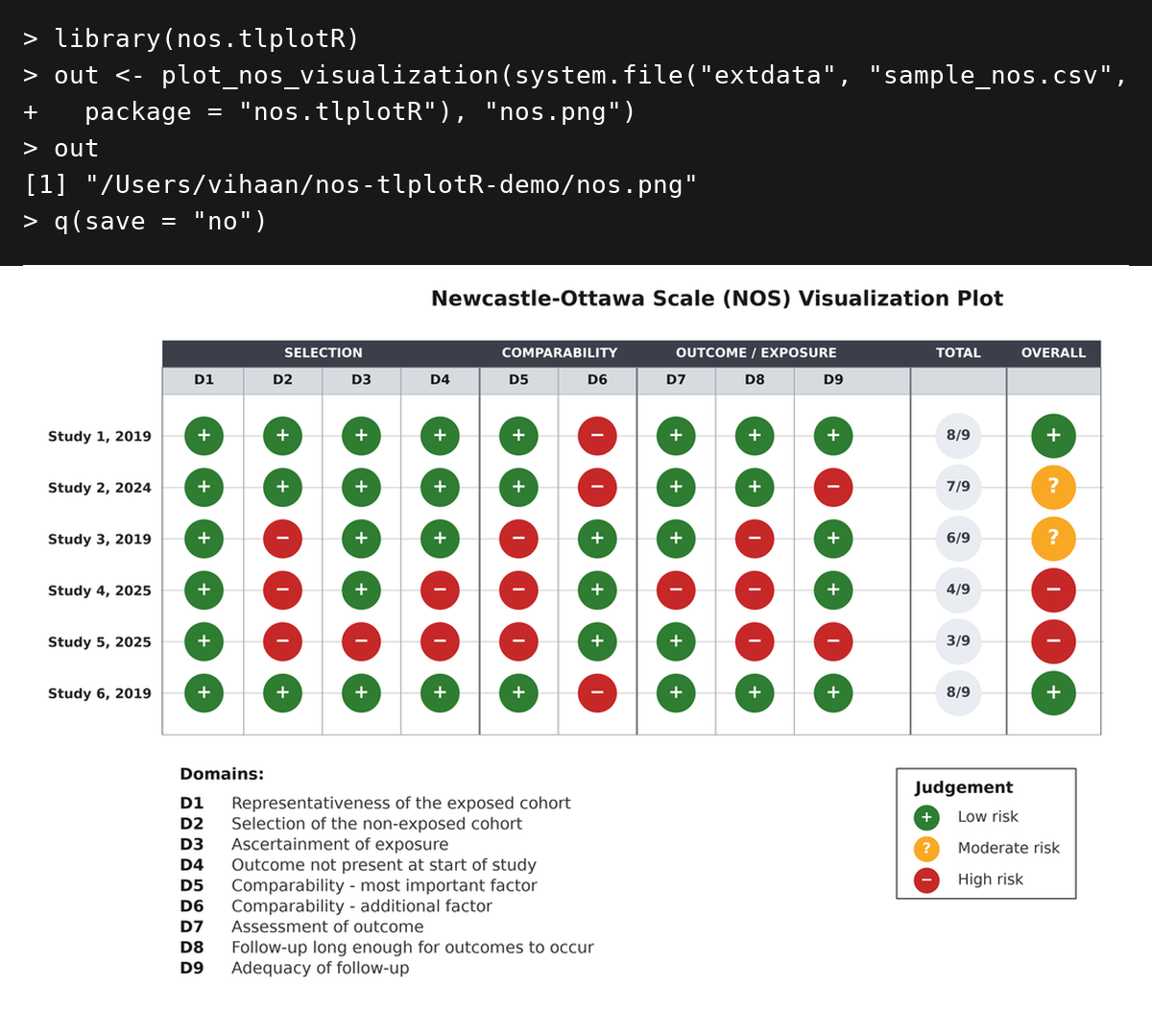
plot_nos_visualization(): item-level traffic-light grid with domain bands, totals and overall judgements.
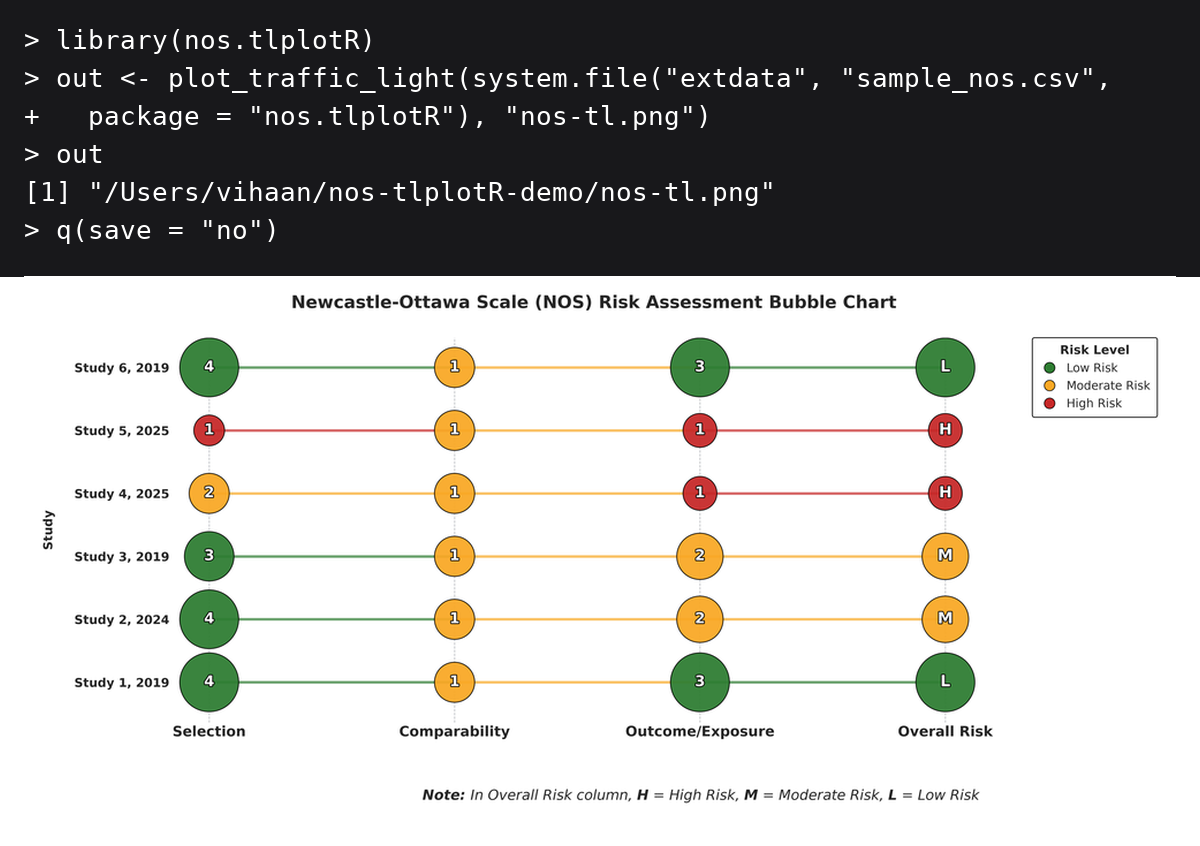
plot_traffic_light().
How to use nos.tlplotR in R
Every plotting function has the same interface:
plot_xxx(input_file, output_file, theme = "traffic_light", verbose = FALSE)-
input_file: a data frame, or a path to a.csv,.xls, or.xlsxfile. -
output_file: path for the plot; the extension must be.png,.pdf,.svg, or.tiff. -
theme: colour theme (see Themes and output formats). -
verbose: ifTRUE, print the messages emitted by the Python package.
Plot from an existing CSV or Excel file
plot_traffic_light(
  input_file  = "my_nos_data.xlsx",
  output_file = "figures/nos.pdf"
)
The output directory must already exist. The package never modifies your input file.
Plot from a data frame
input_file also accepts a data frame, so you can read, filter, or reshape your data in R and pass it straight to a plotting function. The data frame is written to a temporary CSV for Python and removed when the call finishes.
# Read a CSV without mangling the column names
dat <- read.csv("my_nos_data.csv", check.names = FALSE)

# Read an Excel file without mangling the column names
dat <- readxl::read_excel("my_nos_data.xlsx", .name_repair = "minimal")

# Inspect the names before plotting
names(dat)

plot_nos_visualization(dat, "nos.png")
The same works for a subset of studies, a data frame built from scratch, or a tibble:
low_risk <- subset(dat, `Overall RoB` == "Low")
plot_nos_visualization(low_risk, "nos-low.png")
If your column names are already mangled (Overall.RoB instead of Overall RoB), rename them first:
Plot all themes in a loop
input <- system.file("extdata", "sample_nos.csv", package = "nos.tlplotR")

for (theme in c("traffic_light", "gray", "ocean", "sage")) {
  plot_nos_visualization(
    input_file  = input,
    output_file = sprintf("nos-%s.png", theme),
    theme       = theme
  )
}
Generate everything at once
plot_all() mirrors the nos-tlplot command line: one call writes the traffic-light bubble plot to output_file plus the twelve companion figures next to it (_radar, _theme_radar, _heatmap, _item_heatmap, _dot_profile, _table, _donut, _line_ordered, _lollipop, _pie, _stacked_area, _nos_plot), and returns their paths:
files <- plot_all(
  input_file  = system.file("extdata", "sample_nos.csv", package = "nos.tlplotR"),
  output_file = "nos.png"
)

files
#> [1] ".../nos.png"            ".../nos_heatmap.png"
#> [3] ".../nos_item_heatmap.png" "..."
Radar charts are included when there are at most 5 studies and skipped with a message otherwise.
Radar plots and the 5-study limit
Radar charts support at most 5 studies. With more studies no chart is created; the function prints a message and returns NULL invisibly:
res <- plot_domain_radar(input, "radar.png") # NULL when there are > 5 studiesInput data reference
Use the exact names shown below. Column order does not matter.
| Column | Notes |
|---|---|
Author, Year |
One column containing author and year, separated by a comma and space. In a CSV the header must be quoted: "Author, Year". |
Representativeness |
Star value, 0-5 |
Non-exposed Selection |
Star value, 0-5 |
Exposure Ascertainment |
Star value, 0-5 |
Outcome Absent at Start |
Star value, 0-5 |
Comparability (Age/Gender) |
Star value, 0-5 |
Comparability (Other) |
Star value, 0-5 |
Outcome Assessment |
Star value, 0-5 |
Follow-up Length |
Star value, 0-5 |
Follow-up Adequacy |
Star value, 0-5 |
Total Score |
Numeric total, 0-9 |
Overall RoB |
"Low", "Moderate", or "High"
|
💡 Tip: Always include your raw NOS scoring table in supplementary materials for reproducibility.
Themes and output formats
Four colour themes are available on every plot function:
| Theme | Low | Moderate | High |
|---|---|---|---|
traffic_light (default) |
#2E7D32 |
#F9A825 |
#C62828 |
gray |
#D6D6D6 |
#9E9E9E |
#3C3C3C |
ocean |
#6BAED6 |
#2171B5 |
#08306B |
sage |
#63BF93 |
#5B6D80 |
#FF884D |
Supported output formats are PNG (300 dpi), PDF, SVG, and TIFF (LZW compressed). Choose the format through the file extension:
input <- system.file("extdata", "sample_nos.csv", package = "nos.tlplotR")

plot_nos_visualization(input, "nos.png")   # raster, 300 dpi
plot_nos_visualization(input, "nos.pdf")   # vector, for manuscripts
plot_nos_visualization(input, "nos.svg")   # vector, for editing or the web
plot_nos_visualization(input, "nos.tiff")  # LZW-compressed, for journal submission
Return values
All functions return the path of the file they created, invisibly. This makes it easy to chain plotting and reporting:
nos_file <- plot_nos_visualization(
  system.file("extdata", "sample_nos.csv", package = "nos.tlplotR"),
  "nos.png"
)
knitr::include_graphics(nos_file)
They also fail early with a clear R error if the input file is missing, the extension is unsupported, the output directory does not exist, or the theme name is invalid.
Seeing the Python messages
nos-tlplot prints progress and diagnostic messages (for example, warnings about total-score mismatches). These are captured by default so that the functions are silent and work under every locale. Use verbose = TRUE to relay them to the R console:
input <- system.file("extdata", "sample_nos.csv", package = "nos.tlplotR")
plot_traffic_light(input, "nos.png", verbose = TRUE)
Using plots in R Markdown and Quarto
```{r}
library(nos.tlplotR)
plot_nos_visualization(
input_file = "data/nos.csv",
output_file = "figures/nos.png"
)
```
For a figure caption and automatic sizing, use knitr::include_graphics():
Bundled example data
The package ships with a sample NOS dataset in both formats:
list.files(system.file("extdata", package = "nos.tlplotR"))sample_nos.csv sample_nos.xlsxUse them as templates for your own data:
input <- system.file("extdata", "sample_nos.xlsx", package = "nos.tlplotR")
plot_nos_visualization(input, "nos.png")
Troubleshooting
Check the basics first
reticulate::py_config()
reticulate::py_module_available("nos_tlplot")
reticulate::py_run_string("import nos_tlplot; print(nos_tlplot.__file__)")
py_module_available() must return TRUE. If it returns FALSE, Python is either not installed, or the package is installed in a different interpreter than the one reticulate is using.
“The ‘nos-tlplot’ Python package is not available”
Install the module into the interpreter that reticulate uses, then restart R:
reticulate::py_install("nos-tlplot", pip = TRUE)If you use a virtual environment or conda environment, activate it first with reticulate::use_virtualenv() / reticulate::use_condaenv().
reticulate is using the wrong Python
# Temporary, for this session only
Sys.setenv(RETICULATE_PYTHON = "/path/to/python3")

# Permanent
usethis::edit_r_environ()
# add: RETICULATE_PYTHON=/path/to/python3
Restart R after changing RETICULATE_PYTHON. On Windows the path often looks like C:/Users/you/AppData/Local/Programs/Python/Python312/python.exe.
Python is not installed
reticulate::install_python(version = "3.12")Then restart R and check reticulate::py_config() again.
“Missing required columns”
The column names in your file do not match the expected spelling. Common causes:
-
read.csv()replaces spaces with dots in column names. Read withcheck.names = FALSE, or rename the columns. - The author column must be one column named
Author, Year, which has to be quoted in a CSV header:"Author, Year".
Print names(your_data) and compare it with the Input data reference.
XML/Excel errors
Reading .xlsx files needs the Python package openpyxl. It is installed automatically with nos-tlplot, but if you installed nos-tlplot manually:
reticulate::py_install("openpyxl", pip = TRUE)Legacy .xls files are converted in R first and need the readxl package:
install.packages("readxl")If you do not have readxl, save the file as .xlsx or .csv instead.
“Unsupported output file type”
Use .png, .pdf, .svg, or .tiff. Also make sure the output directory already exists and that you have permission to write to it.
Plots are slow the first time
The first call may install Python packages into reticulate’s managed environment. Subsequent calls reuse the cached environment. If you are offline, point reticulate at an interpreter that already has nos-tlplot installed.
Headless Linux server / no display
Matplotlib may try to open a GUI backend. Force the non-interactive backend before Python starts:
Sys.setenv(MPLBACKEND = "Agg")
library(nos.tlplotR)
Still stuck?
Open an issue at https://github.com/nos-tlplot/nos.tlplotR/issues and include the output of:
sessionInfo()
reticulate::py_config()
reticulate::py_module_available("nos_tlplot")
Example gallery
The plots below were generated from the bundled example data (inst/extdata/) with the default theme, using this one-liner pattern:
plot_nos_visualization(
  system.file("extdata", "sample_nos.csv", package = "nos.tlplotR"),
  "nos.png"
)
Flagship plots
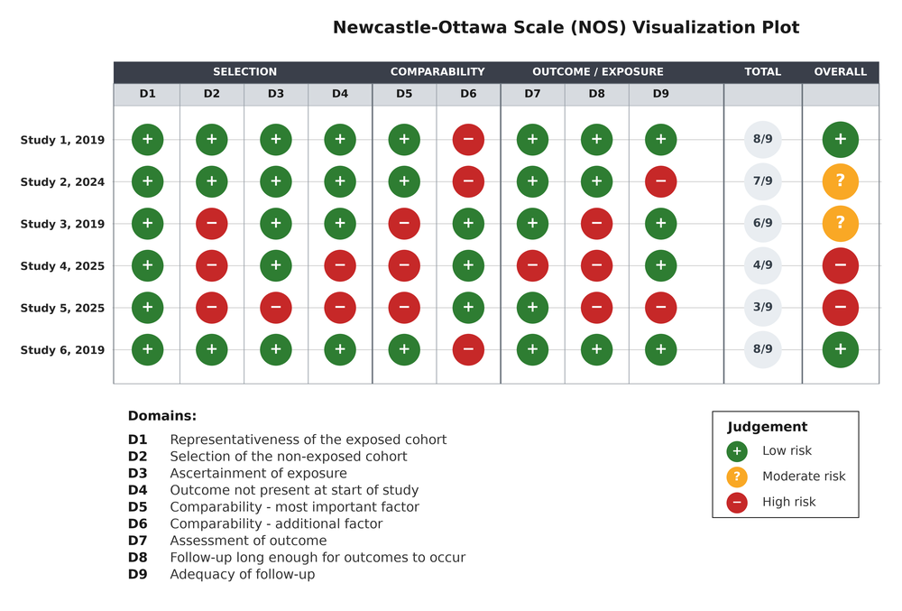
plot_nos_visualization(). One row per study, one column per item, plus totals and the overall judgement.
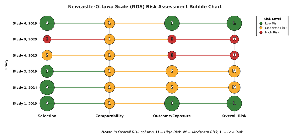
plot_traffic_light(). Bubbles are sized by the stars earned and joined across domains.
Domain-level summaries
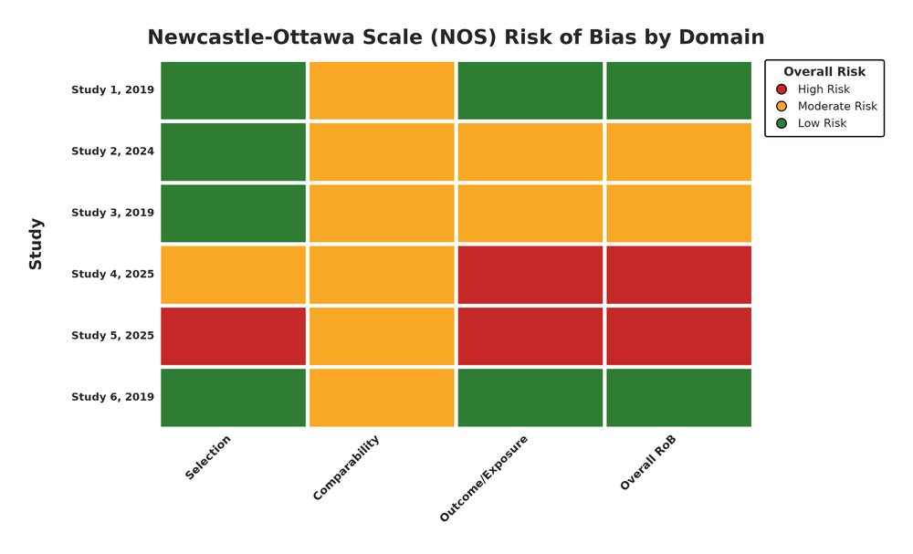
plot_domain_heatmap().
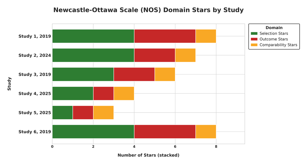
plot_dot_profile().
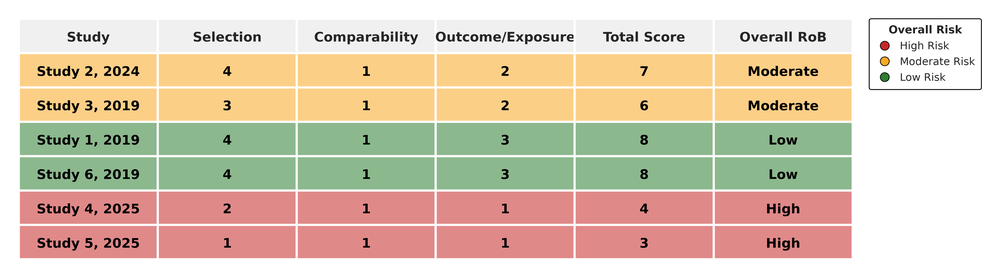
plot_score_table().
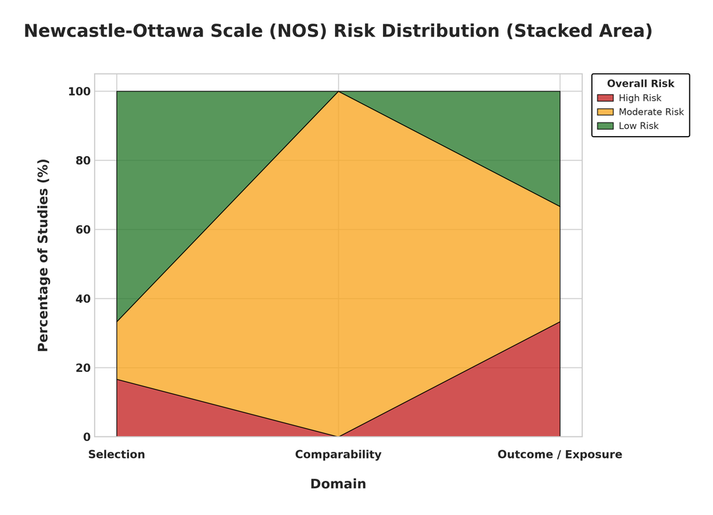
plot_stacked_area().
Item-level plots
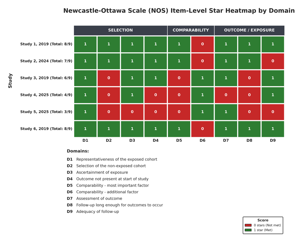
plot_item_heatmap().
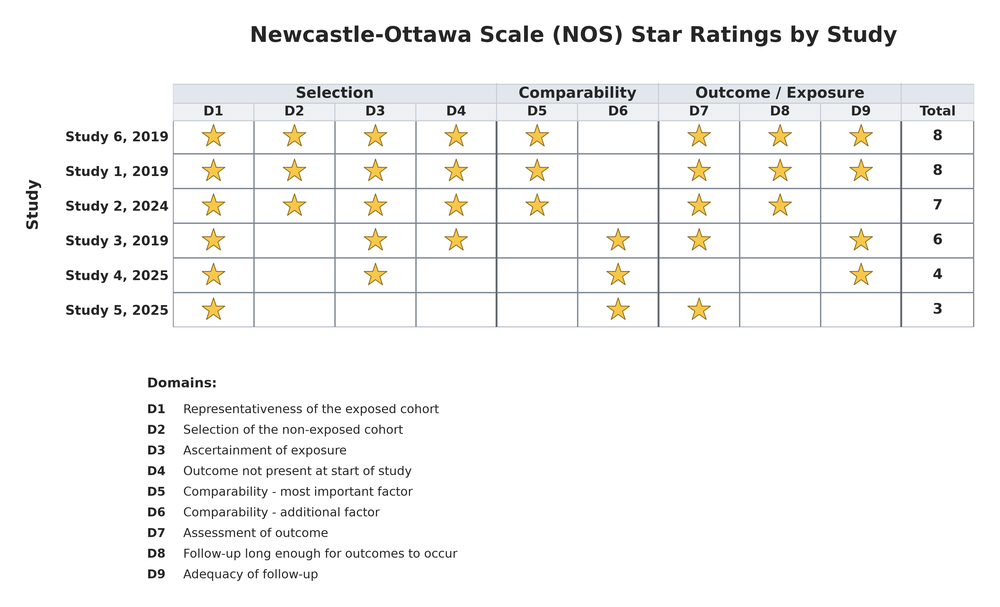
plot_star_matrix().
Distributions
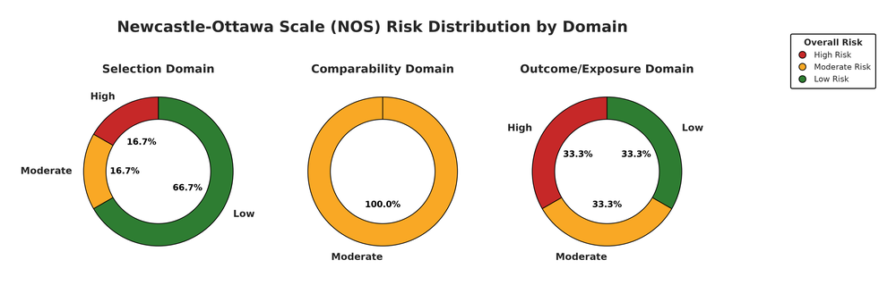
plot_donut().
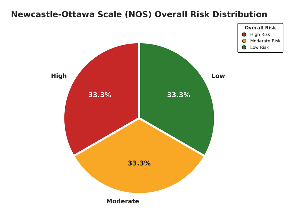
plot_risk_pie().
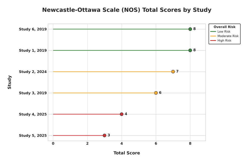
plot_lollipop().
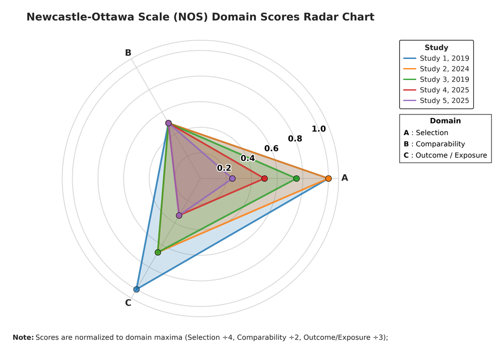
plot_domain_radar(). Radar plots support at most 5 studies.
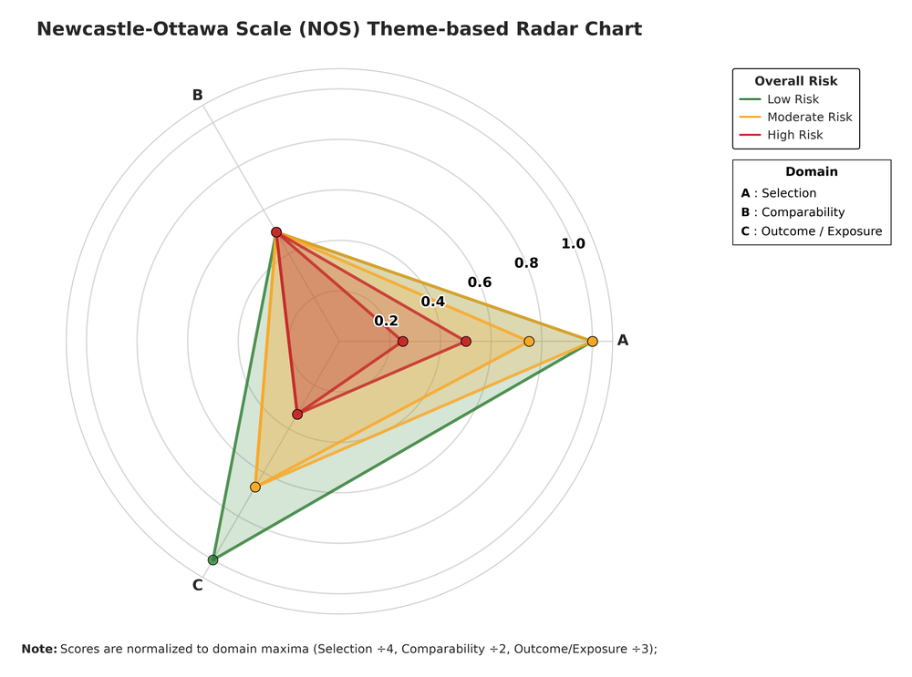
plot_theme_radar().
Theme variants
The same data can be plotted with several colour themes. The NOS visualization above uses the “traffic_light” theme; here are the three alternatives:
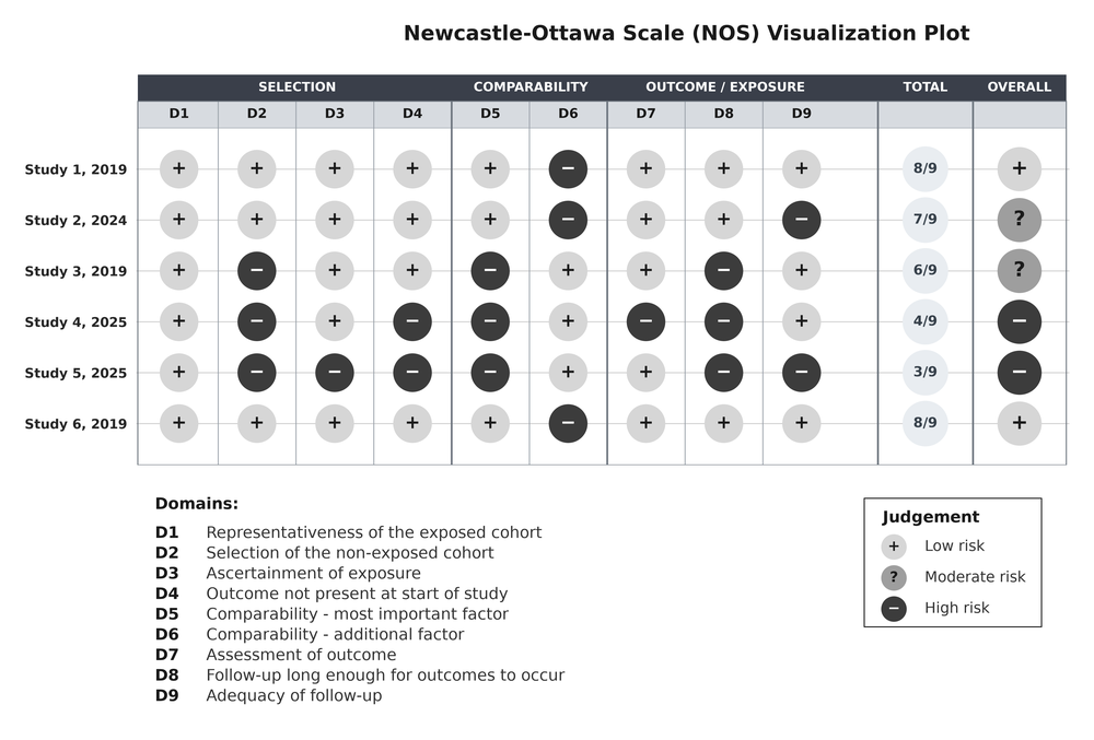
“gray” theme — plot_nos_visualization(…, theme = “gray”).
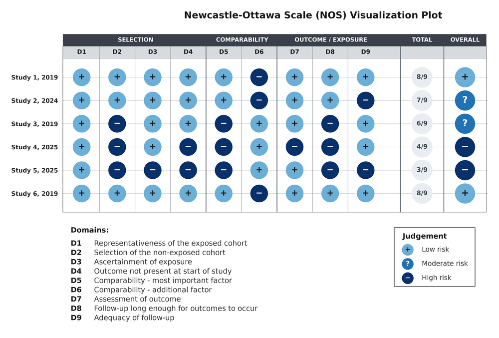
“ocean” theme — plot_nos_visualization(…, theme = “ocean”).
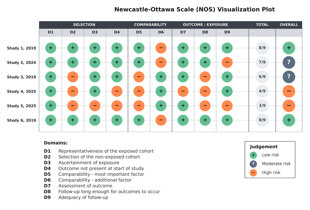
“sage” theme — plot_nos_visualization(…, theme = “sage”).
The full theme list is “traffic_light”, “gray”, “ocean” and “sage” — see Themes and output formats.
Citation
If you use the plots in a publication, the preferred citation is the NOS-TLPlot metapaper:
Sahu, V. (2026). NOS-TLPlot: A Specialized Python Tool for Visualizing Newcastle-Ottawa Scale Risk-of-Bias Assessments. Journal of Open Research Software, 14(1), 7. https://doi.org/10.5334/jors.635
@article{sahu2026jors,
  author = {Sahu, Vihaan},
  title = {NOS-TLPlot: A Specialized Python Tool for Visualizing Newcastle-Ottawa Scale Risk-of-Bias Assessments},
  journal = {Journal of Open Research Software},
  volume = {14},
  number = {1},
  pages = {7},
  year = {2026},
  doi = {10.5334/jors.635},
  url = {https://doi.org/10.5334/jors.635}
}
If you want to cite the code specifically, cite the NOS-TLPlot software:
Sahu, V. (2026). NOS-TLPlot: Visualization Tool for Newcastle-Ottawa Scale in Meta-Analysis (v3.0.2). Zenodo. https://doi.org/10.5281/zenodo.24380517
@software{sahu2026nostlplot,
  author = {Sahu, Vihaan},
  title = {NOS-TLPlot: Visualization Tool for Newcastle-Ottawa Scale in Meta-Analysis},
  year = {2026},
  note = {Version 3.0.2},
  doi = {10.5281/zenodo.24380517},
  url = {https://doi.org/10.5281/zenodo.24380517}
}
and, optionally, the R interface itself:
Sahu, V. (2026). nos.tlplotR: Visualize Newcastle-Ottawa Scale Risk-of-Bias Assessments with ‘nos-tlplot’ (v0.3.0). Zenodo. https://doi.org/10.5281/zenodo.24382618
@software{sahu2026nostlplotr,
  author = {Sahu, Vihaan},
  title = {nos.tlplotR: Visualize Newcastle-Ottawa Scale Risk-of-Bias Assessments with 'nos-tlplot'},
  year = {2026},
  version = {0.3.0},
  doi = {10.5281/zenodo.24382618},
  url = {https://doi.org/10.5281/zenodo.24382618}
}
citation("nos.tlplotR") returns these citations, and the package citation metadata is available at https://github.com/nos-tlplot/nos.tlplotR/blob/main/CITATION.cff.
Related links
- NOS-TLPlot website: https://nos-tlplot.github.io
- Python package on PyPI: https://pypi.org/project/nos-tlplot/
- Python package repository: https://github.com/nos-tlplot/NOS-TLPlot-Package
- Main NOS-TLPlot repository: https://github.com/aurumz-rgb/NOS-TLPlot
- R package repository: https://github.com/nos-tlplot/nos.tlplotR
- reticulate documentation: https://rstudio.github.io/reticulate/
License
Apache License 2.0: https://github.com/nos-tlplot/nos.tlplotR/blob/main/LICENSE.md.